Generalized Backpropagation

Introduction

A neural network computes a function on inputs $\mathbf{x}$ by performing a series of computations propagating information from its inputs to an eventual output $\hat{\mathbf{y}}$; this process is called forward propagation. The error of the network’s output compared to the desired output $\mathbf{y}$ is quantified by a loss function $\mathcal{L}(\mathbf{y}, \hat{\mathbf{y}})$; this error is subsequently allowed to flow backward through the network in the backward propagation step to compute the gradients of all network parameters with respect to the loss function.¹ Precisely, the backward propagation (backpropagation) step is a method of computing gradients of network parameters with respect to a specified loss function; gradient descent is an example of a method that uses these computed gradients as part of a learning paradigm.

The backpropagation algorithm coupled with the stochastic gradient descent training paradigm has seen widespread success in learning numerous neural network architectures; common explicit examples include the feedforward network and the convolutional network. While such derivations provide necessary insight into the workings of such learning algorithms, they ultimately provide narrow glimpses into the general backpropagation framework and lose sight of the forest for the trees.

In this post, we build intution for, derive, and interpret the generalized backpropagation algorithm. The resulting approach, resembling the current methods adopted by popular machine intelligence libaries such as PyTorch and Tensorflow, will enable generalized learning paradigms for a wide variety of network structures (with certain constraints). The material covered in this post is largely inspired and derived from Chapter 6.5 of (Goodfellow et al., 2016); the reader is recommended to refer to the chapter for more examples and clarifying information where necessary.

Fundamental Concepts

Networks as Computational Graphs

It’s useful to formalize the computations performed in a neural network with computational graph language by defining an explicit graph for each network. In particular, each node in our graph will represent a variable (e.g. a scalar, vector, matrix, tensor), and directed edges between nodes will represent operations (functions of one or more variables) between nodes. Our graph will only allow a fixed set of operations for clarity; more complicated functions can be expressed as compositions of operations.

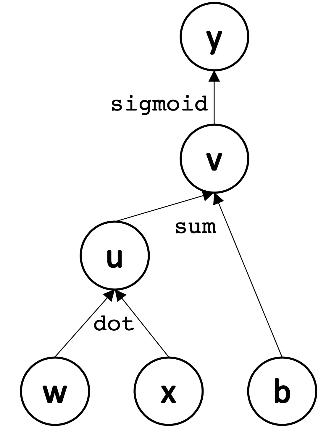
This representation allows us to formally define and reason about operations on neural networks. For example, the forward propagation step begins with observed $\mathbf{x}$ at the leaves of our computational graph. Propagation proceeds layer by layer as nodes perform computation once all their children are observed or have finished computation; as a result, information is propagated through the network to obtain an output and error.

Precisely, let the inputs to a computational graph representation of an arbitrary neural network be $n$ nodes labeled $u^{(1)} \dots u^{(n)}$ and its associated output be $u^{(m)}$. Further let each node compute output $u^{(i)}$ by applying a function $f^{(i)}$ to the set of its parents indexed $j$ such that $j \in Pa(u^{(i)})$. The forward propagation algorithm proceeds as follows:

  
\begin{algorithm}
\caption{Forward propagation algorithm operating on computational graph $G$ with inputs $\mathbf{x}$.}
\begin{algorithmic}

\PROCEDURE{ForwardProp}{$G, \mathbf{x}$}

    \FOR{$i = 1 \dots n$}
    \State $u^{(i)} \gets x_i$
    \ENDFOR 

    \FOR{$i = n + 1 \dots m$}
    \State $P^{(i)} \gets \{u^{(j)} \mid j \in Pa(u^{(i)})\}$
    \State $u^{(i)} \gets f^{(i)}(P^{(i)})$
    \ENDFOR
\ENDPROCEDURE
\end{algorithmic}
\end{algorithm}

We’ll describe backpropagation in a similar vein later in this post.

The Chain Rule of Calculus

The classical chain rule of calculus for one-dimensional variables $x, y, z$ such that $y = g(x)$ and $z = f(y) = f(g(x))$ states that

$$\frac{dz}{dx} = \frac{dz}{dy} \frac{dy}{dx}$$

In order to work with variables of higher dimension in neural networks, we’ll need to generalize this beyond the scalar case. Let $\mathbf{x} \in \mathbf{R}^m, \mathbf{y} \in \mathbf{R}^n, z \in \mathbf{R}$, and let $\mathbf{y} = g(\mathbf{x})$ and $z = f(\mathbf{y}) = f(g(\mathbf{x}))$ for appropriately defined $f, g$. The multivariate chain rule² states that

$$\nabla_\mathbf{x} z = \left( \nabla_\mathbf{y} z \right)^T \left( \frac{\partial \mathbf{y}}{\partial \mathbf{x}} \right) \label{multivar}\tag{1}$$

where

$$\nabla_\mathbf{y} z = \left[ \frac{\partial z}{\partial y_1}, \dots, \frac{\partial z}{\partial y_n} \right]^T$$

is the gradient of $z$ with respect to $\mathbf{y}$ and

$$\frac{\partial \mathbf{y}}{\partial \mathbf{x}} = \begin{bmatrix} \frac{\partial y_1}{\partial x_1} & \frac{\partial y_1}{\partial x_2} & \cdots & \frac{\partial y_1}{\partial x_m} \\ \frac{\partial y_2}{\partial x_1} & \frac{\partial y_2}{\partial x_2} & \cdots & \frac{\partial y_2}{\partial x_m} \\ \vdots & \vdots & \ddots & \vdots \\ \frac{\partial y_n}{\partial x_1} & \frac{\partial y_n}{\partial x_2} & \cdots & \frac{\partial y_n}{\partial x_m} \\ \end{bmatrix}$$

is the Jacobian matrix of $g$ with dimensions $n \times m$. Expanding this matrix multiplication for the derivative of $z$ with respect to a particular $x_i$ yields

$$\frac{\partial z}{\partial x_i} = \sum_j \frac{\partial z}{\partial y_j} \frac{\partial y_j}{\partial x_i} \label{scalar}\tag{2}$$

with the intuitive interpretation that the rate of change of $z$ with respect to $x_i$ depends on all contributions $y_j$ that $x_i$ influences.

Generalizing to Tensors. In order to extend the chain rule to tensors (variables with arbitrary dimension), we can simply flatten each tensor into a vector before running backpropagation, compute vector-valued gradients, and then reshape the gradient back to a tensor. In particular, to denote the gradient of $z$ with respect to tensor $\mathbf{X}$, we write $\nabla_{\mathbf{X}} z$ as if $\mathbf{X}$ were a flattened vector-representation of $\mathbf{X}$. Indices into $\mathbf{X}$, originally tuples of indices across each dimension, can now be represented by a single variable; for all possible index tuples $i$, $(\nabla_{\mathbf{X}} z)_i$ represents $\frac{\partial z}{\partial X_i}$ where $X_i$ is a single scalar value. The chain rule for tensors, where $\mathbf{Y} = g(\mathbf{X})$ and $z = f(\mathbf{Y})$, is therefore

$$\nabla_{\mathbf{X}}z = \left( \nabla_{\mathbf{Y}} z \right)^T \left( \frac{\partial \mathbf{Y}}{\partial \mathbf{X}} \right) = \sum_j \frac{\partial z}{\partial Y_j} \left( \nabla_{\mathbf{X}} Y_j \right) \label{tensor}\tag{3}$$

which is a simple matrix-vector product between the Jacobian $\partial \mathbf{Y} / \partial \mathbf{X}$ and the gradient $\nabla_{\mathbf{Y}} z$.

The Backward Propagation Algorithm

Armed with a computational graph specification and the multivariate chain rule, we’re now ready to understand backward propagation. Recall that the goal of backpropagation is to compute derivatives of the output (loss) function with respect to the parameters of a network. Computing the gradient of a scalar with respect to any node in the computational graph that produced that scalar is relatively simple with the chain rule; indeed, backpropagation is an algorithm that computes the chain rule, but with a specific ordering of operations specified by the associated computational graph that is highly efficient.

To derive the generalized backpropagation algorithm, we’ll first present a simplified version on a scalar graph, and build our way to the general approach accomodating tensor variables.

Working with Scalars

We’ll begin by motivating and presenting the backpropagation algorithm in the simplified case where all variables in our computational graph are scalars. In particular, consider a computational graph with $n$ input nodes labeled $u^{(1)} \dots u^{(n)}$ and output node $u^{(m)}$. To compute the derivative $\frac{\partial u^{(m)}}{\partial u^{(j)}}$ for arbitrary node $u^{(j)}$, the multivariate chain rule (Equation $\ref{scalar}$) yields

$$\frac{\partial u^{(m)}}{\partial u^{(j)}} = \sum_{i \mid j \in Pa(u^{(i)})} \frac{\partial u^{(m)}}{\partial u^{(i)}} \frac{\partial u^{(i)}}{\partial u^{(j)}}$$

We need to perform this computation for every node in our computational graph, but how do we do so efficiently? A naive approach would be to simply compute gradients with respect to nodes $u^{(1)}, u^{(2)}, \dots$ and so on. However, each gradient computation for nodes at the bottom of the computational graph would require re-computing gradients for nodes at higher levels of the graph, making this process inefficient. More precisely, the naive approach would be exponential in the number of nodes, which can be seen by writing the multivariate chain rule explicitly (non-recursively):

$$\frac{\partial u^{(m)}}{\partial u^{(j)}} = \sum_{\text{path } (u^{(\pi_1)}, u^{(\pi_2)}, \dots, u^{(\pi_t)}), \\ \text{ from } \pi_1 = j \text{ to } \pi_t = m} \prod_{k = 2}^t \frac{\partial u^{(\pi_k)}}{\partial u^{(\pi_k - 1)}}$$

Instead, backpropagation exploits the dynamic programming paradigm to compute gradients in an efficient manner that eliminates the burden of re-computing common, expensive gradients at each application of the chain rule.³ Instead of starting computation at the bottom of the graph, backpropagation begins at the output nodes, computing and storing gradients while traversing through the computational graph in a reverse direction (hence the name backpropagation).

More precisely, backpropagation operates on a modified computational graph $G’$ which contains exactly one edge $u^{(i)} \to u^{(j)}$ for each edge from node $u^{(j)} \to u^{(i)}$ of the original graph $G$; this edge is associated with the computation of $\frac{\partial u^{(i)}}{\partial u^{(j)}}$ and its multiplication with the gradient already computed for $u^{(i)}$ (that is, $\frac{\partial u^{(m)}}{\partial u^{(i)}}$). As a result, each edge in $G’$ computes the blue portion of our earlier expression of the multivariate chain rule, and the sum of all incoming edges to each node in $G’$ computes the red portion, yielding our desired result.

$$\frac{\partial u^{(m)}}{\partial u^{(j)}} = \color{red}{\sum_{i \mid j \in Pa(u^{(i)})}} \color{blue}{\frac{\partial u^{(m)}}{\partial u^{(i)}} \frac{\partial u^{(i)}}{\partial u^{(j)}}}$$

This order of operations allows backpropagation to scale linearly with the number of edges in $G$, avoiding repeated computations. Specifically, to compute the gradient of an output node with respect to any of its ancestors (say, $a$) in computational graph $G$, we begin by noting that the gradient of the output node with respect to itself is 1. We then compute the gradient of the output node with respect to each of its parents in $G$ by multiplying the current gradient with the Jacobian of the operation that produced the output (in the scalar case, this is simply the partial of the output with respect to the input). We continue doing so, summing gradients for nodes that have multiple children in $G$, until we reach $a$.

Working with Tensors

Now that we’ve discussed backpropagation in the scalar case, let’s generalize to tensor-valued nodes. Our logic here will follow the same process summarized at the end of the prior section, but will employ a bit more formalism to encapsulate the most general case.

Formally, each node in $G$ will correspond to a variable as before, but we now allow variables to be tensors (which, in general, can have an arbitrary number of dimensions). Each variable $V$ is also associated with the operations

• get_operation(V), which returns the operation that computes $V$ as represented by the edges incident on $V$ in $G$.
• get_children(V, G), which returns the list of children of $V$ in $G$.
• get_parents(V, G), which returns the list of parents of $V$ in $G$.

Each operation op(inputs) returned by get_operation(V) is associated with a backpropagation operation op.bprop(inputs, var, grad) for each of op’s input arguments, which computes the Jacobian-gradient product specified in Equation \ref{tensor}. In particular, op.bprop(inputs, X, G) returns

$$\mathbf{G}^T \nabla_\mathbf{X} \texttt{op(inputs)} = \sum_j G_j (\nabla_\mathbf{X} \texttt{op(inputs)}_j )$$

where $\mathbf{G}$ is the gradient of the final computational graph output with respect to the output of op and $\mathbf{X}$ is the input variable to op which we are computing gradients with respect to.

As a quick example to solidify intuition, let op(inputs = [A, B]) = $AB$ be the matrix product of two tensors $A$ and $B$. This operation also defines

• op.bprop(inputs, A, G) = $A^TG$
• op.bprop(inputs, B, G) = $GB^T$

which specify the gradients of the operation with respect to each of the inputs. Note that op must treat each of its inputs as distinct, even if $A = B$; this is because these individual gradients will eventually be added to obtain the correct total.

The formal backpropagation algorithm thus proceeds as follows.

  
\begin{algorithm}
\caption{Backward propagation algorithm operating on computational graph $G$ with output $z$ and target variables for gradient computation $T$.}
\begin{algorithmic}

\PROCEDURE{BackwardProp}{$G, T, z$}

    \State $G' \gets G$ with only nodes that are ancestors of $z$ and descendants of nodes in $T$
    \State $\texttt{grad\_table} \gets []$ \Comment{A data structure associating tensors to their gradients}
    \State $\texttt{grad\_table}[z] \gets 1$
    
    \For{$\mathbf{V} \in T$}
    \State $\texttt{BuildGradient}(V, G', \texttt{grad\_table})$
    \EndFor
    
    \Return $\texttt{grad\_table}$ restricted to elements in $T$
\ENDPROCEDURE
\end{algorithmic}
\end{algorithm}

The meat of the work happens in the $\texttt{BuildGradient}$ subroutine, as follows.

  
\begin{algorithm}
\caption{Backward propagation algorithm subroutine to compute the gradient for variable $V$ on a computational graph restriction to participating nodes $G'$, with data structure mapping nodes to gradients $\texttt{grad\_table}$.}
\begin{algorithmic}

\PROCEDURE{BuildGradient}{$V, G', \texttt{grad\_table}$}

    \If{$V$ is in $\texttt{grad\_table}$}
    \Return $\texttt{grad\_table}[V]$
    \EndIf

    \State $i \gets 1$
    
    \For{$C \in \texttt{get\_children}(V, G')$} \Comment{Sum gradient contributions from children of $V$ in $G'$}
        \State{$\texttt{op} \gets \texttt{get\_operation}(C)$}
        \State{$C_{grad} \gets \texttt{BuildGradient}(C, G', \texttt{grad\_table})$} \Comment{This computes $\partial z / \partial C$}
        \State{$G^{(i)} \gets \texttt{op.bprop(get\_parents(C, G'), V, } C_{grad} \texttt{)}$} \Comment{This computes $\partial z / \partial C \times \partial C / \partial V $}
        \State{$i \gets i + 1$}
    \EndFor

    \State{$G \gets \sum_i G^{(i)}$} \Comment{Sum incoming gradients}
    \State{$\texttt{grad\_table}[V] \gets G$}

    \Return $G$
\ENDPROCEDURE
\end{algorithmic}
\end{algorithm}

Note that lines 6 - 11 operate in a backwards propagating manner as previously described; no gradients are computed until a previously known gradient is obtained (which is initially only the output node of the graph), and subsequent computations proceed backward along $G’$, summing computations for the children of $V$ until the final gradient is computed (and stored in the gradient table for later calls). This table-filling aspect of backpropagation which allows the algorithm to avoid repeating common subexpressions is what makes it a dynamic programming approach.

Conclusion and Further Considerations

Backpropagation is a fundamental algorithm for the computation of gradients of variables in computational graphs in a highly efficient manner. When coupled with an optimization algorithm (often stochastic gradient descent) for adjusting parameters based on their gradients with respect to an output, backpropagation enables the fast and efficient training of an amalgam of neural networks. It does so by following the dynamic programming paradigm to store intermediate gradients in a table and performing computations backwards in the computational graph, thereby avoiding the exponential complexity of a naive approach and instead requiring linear time in the number of edges in the graph.

While the algorithm described in this post is general (and is similar to the symbol-to-number approach employed in PyTorch), it papers over many complexities that arise when designing real-world generalized backpropagation routines. Indeed, our approach only applies to operations that return a single tensor; many implementations must allow for operations to return more than one tensor. Additionally, while backpropagation reduces the time complexity of gradient computation, it comes with a linear memory cost, which can be prohibitive in large comuptational graphs. The solutions to these and other subtelties are at the core of libraries such as PyTorch and Tensorflow, which are able to enable gradient computation at scale.

Notes