Learning Feedforward Networks

There’s no lack of tutorials on feedforward (“neural”) networks and their learning algorithms, but I’ve often found that online resources often leave many details to the reader or employ confusing notation without providing relevant intuition. Here, I methodically derive backpropagation for feedforward networks. This post was inspired by, and some of its content was derived from, these two excellent resources.

Introduction and Notation

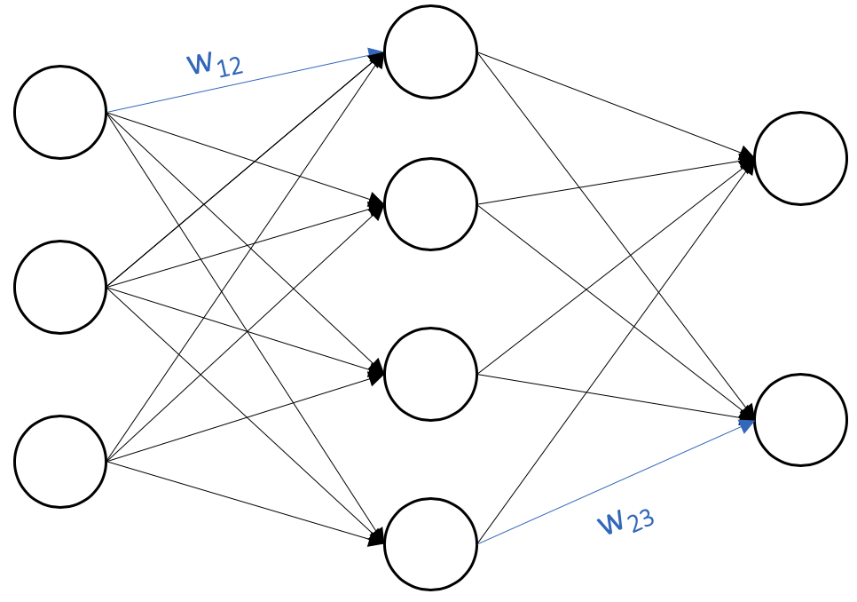
For the duration of this post, we’ll consider a feedforward network with $L$ layers indexed $l = 1 \dots L$ as in the diagram below. Each node in a feedforward network computes a weighted output and an activation. Intuitively, a node’s weighted output sums and weights information from nodes in the previous layer, and its activation applies a nonlinearity to the weighted output so that the network can compute nonlinear functions.

Feedforward networks have three types of nodes:

• Input nodes ($l = 1$), whose weighted outputs are fixed by the input values
• Hidden nodes ($l = 2 \dots L - 1)$, whose weighted inputs are determined by a linear combination of the previous nodes’ activations
• Output nodes ($l = L$), whose activations are treated as the predictions of the network

Each node $i$ in layer $l$ is associated with weights $w_{ij}$ for all connections to nodes $j$ in layer $l+1$ along with a bias $b_i$. Figure 1 provides a visual diagram of a three-layer network, with one input layer, one hidden layer, and one output layer.

Now that we can visualize feedforward networks, let’s dive into the math. Precisely, consider a dataset of pairs $(x, y)$. Nodes in layer $l$ compute weighted outputs

$$\begin{align} z_i^l = \begin{cases} x_i & l = 1 \\ \sum_j w_{ji}^l a_j^{l-1} + b_i^l & \text{else} \end{cases} \end{align}$$

and activations

$$a_i^l = \sigma(z_i^l)$$

where subscripts denote indices within a layer, superscripts denote layer indices, and $\sigma(\cdot)$ is some nonlinearity. In simpler terms, node weighted outputs are either the network inputs in the first layer or a linear combination of the previous layer’s activations for all other layers. As mentioned before, activations introduce nonlinearities into the network.

Ideally, we’d like the outputs of our network operating with input $x$ to be as close to the true label $y$; we quantify our success with a loss function $\mathcal{L}(a^L, y)$. Feedforward networks require two assumptions on the loss function for stochastic gradient descent:

1. The loss function can be written as an average $\mathcal{L} = \frac{1}{n} \sum \mathcal{L}_x$ for individual training examples $x$

2. The loss function can be written as a function of the outputs of the feedforward network, so that the derivative $\partial \mathcal{L}(a^L, y) / \partial a^L$ depends only on $a^L$.

Cross-entropy is a typical loss function for classification problems, and mean squared error is typical for regression problems.

Forward Propagation

Forward propagation is the process of forwarding an input $x$ through a feedfoward network to produce outputs $a^L$. We may compute these outputs systematically as follows:

1. Compute the activations of the input layer: for each $i$, compute $a_i^1 = \sigma(x_i)$

2. Compute the activations of all remaining layers in order: for $l = 2 \dots L$, compute

$$a_i^l = \sigma \left( \sum_j w_{ji}^l a_j^{l-1} + b_i^l \right)$$

where the sum is over all nodes $j$ in layer $l-1$. We now see why this process is called “forward propagation”: computation propagates from the first layer to the final layer in the network. Note that we can write step (2) in terms of matrix operations to speed up computation; if we treat the nonlinearity $\sigma$ as an elementwise operator, we have that

$$\mathbf{a}^l = \sigma \left( \mathbf{w}^{T^l} \mathbf{a}^{l-1} + \mathbf{b}^l \right)$$

If you’re having trouble with the transpose, consider an example with $n$ nodes in the input layer $l-1$ and $m$ nodes in the output layer. By definition, we have $\mathbf{w}^l \in \mathbf{R}^{n \times m}, \mathbf{a}^{l-1} \in \mathbf{R}^{n \times 1}, \mathbf{b}^l \in \mathbf{R}^{m \times 1}$. For the multiplication to work out (yielding output $\mathbf{a}^l \in \mathbf{R}^{m \times 1}$), we need the transpose.

Backward Propagation

Now that we know how to obtain an output from our network, the next step is to update the parameters (weights and biases) of the network to yield a desirable output as per the loss function $\mathcal{L}$. A classical way to do so is to update each parameter in the negative direction of its gradient with respect to $\mathcal{L}$; this would achieve the global minimum of $\mathcal{L}$ for convex $\mathcal{L}$, but does reasonably well in non-convex cases as well.

It’s easy to estimate the gradients of $\mathcal{L}$ with respect to each weight and bias empirically. Specifically, let $\mathcal{L}’(x)$ be the loss value with $w_{ji}^{l’} \leftarrow w_{ji}^l + \delta$; we can compute

$$\frac {\partial \mathcal{L}}{\partial w_{ji}^l} \approx \frac{\mathcal{L}'(x) - \mathcal{L}(x)}{\delta}$$

and update $w_{ji}^l = w_{ji}^l - \gamma \frac {\partial \mathcal{L}}{\partial w_{ji}^l}$ for some small, fixed learning rate $\gamma$. But there are obvious problems with this approach: we’d have to perform forward propagation once for every weight (and bias) in the network, an extremely expensive process.

Backward propagation attempts to remedy such computational inefficiencies by updating weights in one backward pass through the network. To do so, we make extensive use of the chain rule. Let’s start by computing partials of the loss function with respect to the network weights and biases. We can write

$$\begin{align} \frac{ \partial \mathcal{L}}{\partial w_{ji}^l} &= \frac{\partial \mathcal{L}}{\partial z_i^l} \frac{\partial z_i^l}{\partial w_{ji}^l} \\ \frac{ \partial \mathcal{L}}{\partial b_{i}^l} &= \frac{\partial \mathcal{L}}{\partial z_i^l} \frac{\partial z_i^l}{\partial b_i^l} \end{align}$$

where we take the partial with respect to $z_i^l$ as $z_i^l = \sum_j w_{ji}^l a_j^{l-1} + b_i^l$. Since we have an explicit relationship between $z_i^{l+1}$ and $w_{ji}^l$, we can write

$$\boxed{ \frac{ \partial \mathcal{L}}{\partial w_{ji}^l} = \frac{\partial \mathcal{L}}{\partial z_i^l} a_j^{l-1} }$$

and

$$\boxed{ \frac{ \partial \mathcal{L}}{\partial b_i^l} = \frac{\partial \mathcal{L}}{\partial z_i^l} }$$

In both cases, we’ll need to compute $\partial \mathcal{L} / \partial z_i^l$. We can express

$$\frac{\partial \mathcal{L}}{\partial z_i^l} = \frac{ \partial \mathcal{L}}{\partial a_i^l} \frac{\partial a_i^l}{\partial z_i^l}$$

where we take the partial with respect to $a_i^l$ as $a_i^l = \sigma(z_i^l)$. Since we have an explicit relationship between $a_i^l$ and $z_i^l$, we can write

$$\boxed{ \frac{\partial \mathcal{L}}{\partial z_i^l} = \frac{ \partial \mathcal{L}}{\partial a_i^l} \sigma'(z_i^l) }$$

Finally, we have to deal with the $\partial \mathcal{L} / \partial a_i^l$ term; this is where the “backpropagation” term comes into play. Note that for $l = L$, we know that the partial is just a derivative of $\mathcal{L}(a^L, y)$, which we can analytically compute. Now for a layer $l \neq L$, we have that

$$\frac{\partial \mathcal{L}}{\partial a_i^l} = \sum_k \frac{\partial \mathcal{L}}{\partial z_k^{l+1}} \frac{\partial z_k^{l+1}}{\partial a_i^l}$$

where we take the partial with respect to all $z_k^{l+1}$ in the subsequent layer as all such terms depend on the activation $a_i^l$ via the relationship $z_k^{l+1} = \sum_j w_{jk}^{l+1} a_j^l + b_k^{l+1}$. Since we have an explicit relationship between $z_k^{l+1}$ and $a_i^l$, we can write

$$\boxed{ \frac{\partial \mathcal{L}}{\partial a_i^l} = \sum_k \frac{\partial \mathcal{L}}{\partial z_k^{l+1}} w_{ji}^{l+1} }$$

Since we can compute $\partial \mathcal{L} / \partial z_k^L$, and since every layer’s partials depend on the layer after it, all that’s left to do is sequentially iterate backward through the network, computing partials as we go—hence, backward propagation.

The Backprop Algorithm

Our algorithm thus proceeds as follows. We begin by compute the partial derivatives of the loss function with respect to the activations of the final layer ($L$); this is $\partial \mathcal{L} / \partial a_i^L$.

For layers $l = L \dots 1$ (all layers aside from the input), we:

1. Compute the partial derivative of the loss function with respect to node inputs

   $$\frac{\partial \mathcal{L}}{\partial z_i^l} = \frac{ \partial \mathcal{L}}{\partial a_i^l} \sigma'(z_i^l)$$

   If we treat $\sigma( \cdot )$ as an elementwise operator and $\odot$ as the Hadamard (elementwise) matrix product, we can write this step as

   $$\frac{\partial \mathcal{L}}{\partial \mathbf{z}^l} = \frac{ \partial \mathcal{L}}{\partial \mathbf{a}^l} \odot \sigma'(\mathbf{z}^l)$$

2. Backpropagate the error: compute the partial derivative of the loss function with respect to the activations of the previous layer

   $$\frac{\partial \mathcal{L}}{\partial a_i^{l-1}} = \sum_k \frac{\partial \mathcal{L}}{\partial z_k^l} w_{ji}^l$$

   This step can be written in terms of matrix operations as

   $$\frac{\partial \mathcal{L}}{\partial \mathbf{a}^{l-1}} = \left(\mathbf{w}^{T^l} \right) \frac{\partial \mathcal{L}}{\partial \mathbf{z}}$$

   Note that since there’s no layer to backpropagate error to for $l = 1$, we don’t perform this step for the input layer.

We now have $\partial \mathcal{L} / \partial a_i^l$ for all layers $l$, and so we can compute the partial derivatives for all weights and biases, completing our update.