Learning Convolutional Networks

Many courses in machine intelligence often cover backpropagation for feedforward networks, and claim that a similar approach can be applied to convolutional networks without any additional justification. Here, I methodically derive backpropagation for convolutional networks. The notation used and general structure of this post is similar to my derivation of backpropagation for feedforward networks, which functions as an excellent introduction to backpropagation if the reader is not familiar with such concepts.

Introduction and Motivation

Consider a dataset of images of handwritten digits $x$ and associated digit values $y$. Since we’re now dealing with multimensional images as input instead of a single-dimensional set of features, one solution is to “flatten” each $l \times w \times h$ image into an $lwh$-length input array for a feedfoward network. While such a pipeline would work and provide reasonable results (De Chazal et al., 2015), it treats each pixel of the image as independent and destroys structural features, significantly diminishing prediction quality.

Convolutional networks, proposed in (LeCun et al., 1999) and popularized by (Krizhevsky et al., 2012), provide a powerful way to train networks with desirable inductive biases for image classification problems. In particular, convolutional networks employ three basic ideas—local receptive fields, shared weights, and pooling—to preserve and utilize structural features for prediction. We’ll discuss each in turn, developing intuition for the structure of a convolutional network in the process.

Local receptive fields. While feedforward networks consist of a single layer of input nodes that are fully connected to hidden layer nodes, convolutional networks treat the input as a multidimensional array and connect hidden nodes to a small region of the input nodes (as illustrated in Figure 1). This small region of nodes, called the local receptive field of a node in the subsequent layer, is slid across the input layer, with each new field connecting to a new output node. As in feedforward networks, each connection learns a weight, and each hidden node learns a bias as well.

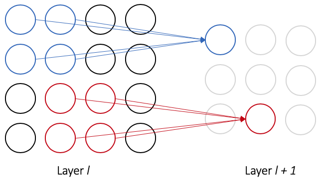
Shared weights. Now that we understand connections as they relate to local receptive fields in convolutional networks, we can introduce the concept of shared weights. While the general form of Figure 1 allows each connection to learn its own weight, convolutional networks impose the constraint that all nodes in layer $l + 1$ share the same weights and bias. In Figure 1, this implies that the $j, k$th hidden node has output

$$a^{l+1}_{j, k} = \sigma \left( \sum_{a = 0}^1 \sum_{b = 0}^1 w^{l+1}_{a, b} a^l_{j + a, k + b} + b^{l+1} \right)$$

where $w^{l+1}$ is the shared weight matrix, $a^l$ defines the input activations from layer $l$ to layer $l + 1$, and $b^{l+1}$ is the shared bias for layer $l$. This output equation is the exact same as that of convolutional networks, but altered to share weights and only use information from a node’s local receptive field. It turns out that the output equation is identical to that of a discrete convolution, which gives convolutional networks their name.

Shared weights (also called “feature maps” or “filters”) are useful because they allow all nodes in a given hidden layer to detect the same input pattern (perhaps an edge in the image, or a particular kind of shape) at different areas of the input image. As a result, convolutional networks preserve structural and translational invariance of images.

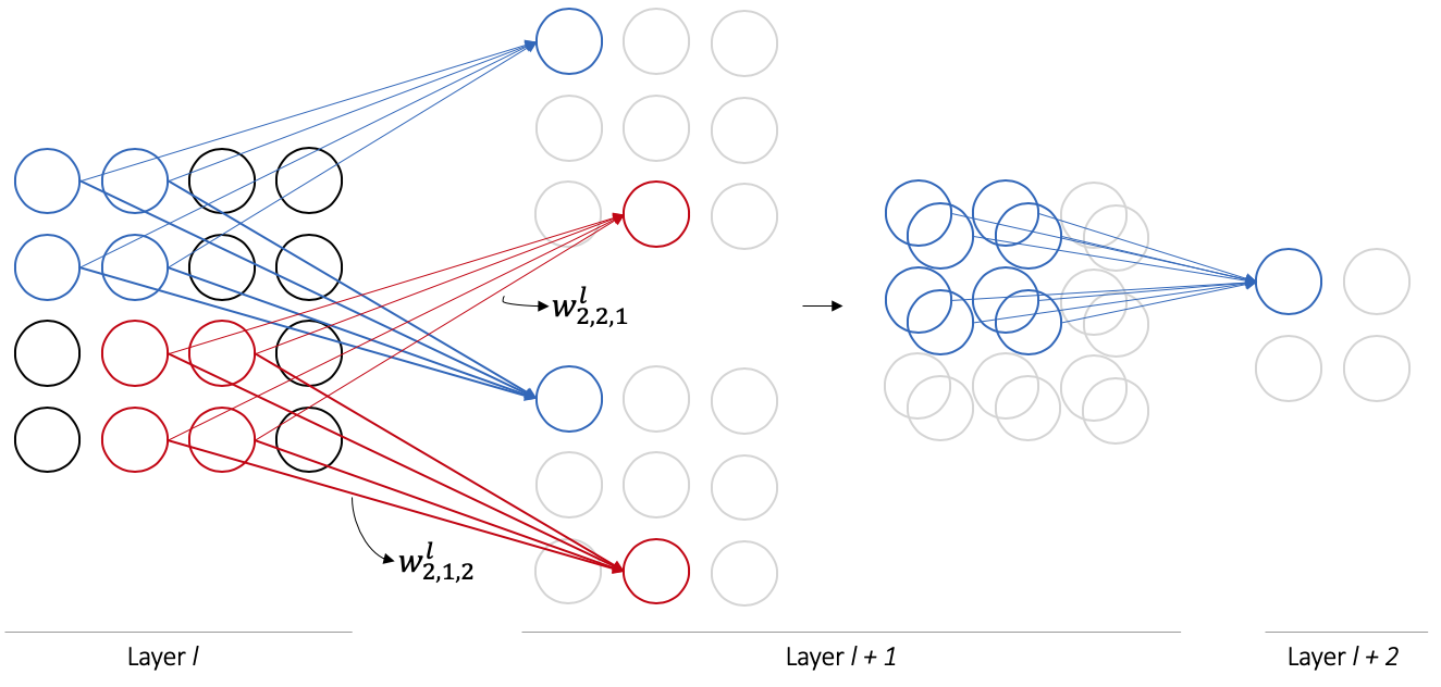
While our current network in Figure 1 only allows layer $l + 1$ to learn one set of shared weights (one feature map), convolutional networks often employ multiple sets of feature maps per layer as in Figure 2. This allows for more expressive power per layer; the multiple outputs produced are concatenated along a new dimension and passed as input to the next hidden layer.

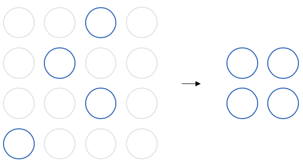
Pooling layers. Convolutional networks additionally employ pooling layers to reduce the number of nodes involved as the network grows deeper. Pooling layers are quite simple: they subsample blocks of nodes from a layer to produce a single output, reducing the size of the layer as output. The most common pooling operation is called maximum pooling, which selects the maximum value of its input nodes for its output (as in Figure 3).

Convolutional networks utilize a combination of local receptive fields, shared weights, and pooling layers to define their architectures. In particular, canonical architectures consist of an input layer followed by some number of convolutional and pooling layers, followed by some number of fully connected layers, followed by an output layer. General architectural patterns along with samples are located here.

Forward Propagation

With our knowledge of convolutional network architectures, we can precisely define forward propagation.

Convolutional Layers. Here, we consider convolutional layers (which utilize local receptive fields and shared weights) along three dimensions with multiple feature maps, as most images are three-dimensional and learning multiple feature maps from an input produces a three-dimensional output. However, there are obvious generalizations of our discussion to higher (or lower)-dimensional networks.

Let the input to our convolutional layer be $\mathbf{a}^{l - 1} \in \mathbf{R}^{r \times s \times t}$, and let feature map $m$ (of $M$ total) be parameterized as $\mathbf{w}^{l, m} \in \mathbf{R}^{d \times d \times t}$, where the third dimension of the feature map matches the third dimension of the input. The weighted output of our convolutional layer is $\mathbf{z}^l \in \mathbf{R}^{(r - d + 1) \times (s - d + 1) \times M}$. We can write the weighted output for feature map $m$ as

$$z^{l}_{i, j, m} = \sum_{a = 0}^{d-1} \sum_{b = 0}^{d-1} \sum_{c = 0}^{t - 1} w^{l, m}_{a, b, c} a^{l-1}_{(i + a), (j + b), c} + b^{l,m}$$

which is effectively a discrete convolution between the (shared) weight matrix and the relevant slice of the input nodes. The activations are thus

$$a^{l}_{i, j, m} = \sigma (z_{i, j, m}^{l})$$

for some nonlinearlity $\sigma (\cdot )$.

(Maximum) Pooling Layers. Maximum pooling layers are quite straightforward; they only select the largest value within each $k \times k$ region in an input, and output the resulting layer with reduced size.

That’s it! Let’s now move on to deriving the backpropagation rules for these layer updates. We’ll follow a similar procedure to the derivation for feedfoward networks here.

Backward Propagation

Now that we know how to obtain an output from our network, the next step is to update the parameters (weights and biases) of the network to yield a desirable output as per the loss function $\mathcal{L}$.

Convolutional Layers. Let’s start by computing partials of the loss function with respect to the network weights and biases. For weight $w^{l, m}_{a, b, c}$ at layer $l$ in feature map $m$ and bias $b^l$, we have

$$\begin{align} \frac{\partial \mathcal{L}}{w^{l, m}_{a,b,c}} &= \sum_{i = 0}^{r - d} \sum_{j = 0}^{s - d} \frac{\partial \mathcal{L}}{\partial z_{i,j,m}^l} \frac{\partial z_{i,j,m}^l}{\partial w^{l, m}_{a,b,c}} \\ \frac{\partial \mathcal{L}}{b^{l, m}} &= \sum_{i = 0}^{r - d} \sum_{j = 0}^{s - d} \frac{\partial \mathcal{L}}{\partial z_{i,j,m}^l} \frac{\partial z_{i,j,m}^l}{\partial b^{l, m}} \end{align}$$

where we assume $w$ is a $d \times d \times t$ feature map and layer $l$ has dimensions $r \times s \times t$. The summations are involved as we must sum over all weighted output expressions that contain $w^{l, m}_{a,b,c}$—this corresponds to weight sharing in the convolutional network.

Since we have an explicit relationship between $z_{i,j, m}^l$ and $w_{a,b,c}^{l,m}$, we can write

$$\boxed{\frac{\partial \mathcal{L}}{w^{l, m}_{a,b,c}} = \sum_{i = 0}^{r - d} \sum_{j = 0}^{s - d} \frac{\partial \mathcal{L}}{\partial z_{i,j,m}^l} a^{l-1}_{(i + a), (j + b), c} }$$

and

$$\boxed{\frac{\partial \mathcal{L}}{b^{l, m}} = \sum_{i = 0}^{r - d} \sum_{j = 0}^{s - d} \frac{\partial \mathcal{L}}{\partial z_{i,j,m}^l}}$$

In both cases, we’ll need to compute $\frac{\partial \mathcal{L}}{\partial z_{i,j,m}^l}$. We can express

$$\frac{\partial \mathcal{L}}{\partial z_{i,j,m}^l} = \frac{\partial \mathcal{L}}{\partial a_{i,j,m}^l} \frac{\partial a_{i,j,m}^l}{\partial z_{i,j,m}^l}$$

where we take the partial with respect to $a_{i,j,m}^l$ as $a_{i,j,m}^l = \sigma(z_{i,j,m}^l)$. Since we have an explicit relationship between $a_{i,j,m}^l$ and $a_{i,j,m}^l$, we can write

$$\boxed{\frac{\partial \mathcal{L}}{\partial z_{i,j,m}^l} = \frac{\partial \mathcal{L}}{\partial a_{i,j,m}^l} \sigma'(z_{i,j,m}^l) }$$

Finally, we have to deal with the $\partial \mathcal{L} / \partial a_{i,j,m}^l$ term; this is where the “backpropagation” term comes into play. For the final layer in the network, we can analytically compute this term as $\mathcal{L}$ is a function of the activations of the last layer. For all other layers, we have that

$$\frac{\partial \mathcal{L}}{\partial a_{i,j,m}^l} = \sum_{a = 0}^{d'-1} \sum_{b = 0}^{d'-1} \sum_{k = 0}^K \frac{\partial \mathcal{L}}{\partial z_{(i-a),(j-b),k}^{l+1}} \frac{\partial z_{(i-a),(j-b),k}^{l+1}}{\partial a_{i,j,m}^l}$$

where we assume $w^{l+1}$ is a $d’ \times d’ \times M$ feature map and layer $l+1$ uses $K$ feature maps. Since we have an explicit relationship between $z_{(i-a),(j-b),k}^{l+1}$ and $a_{i,j,m}^l$, we can write

$$\boxed{\frac{\partial \mathcal{L}}{\partial a_{i,j,m}^l} = \sum_{a = 0}^{d'-1} \sum_{b = 0}^{d'-1} \sum_{k = 0}^K \frac{\partial \mathcal{L}}{\partial z_{(i-a),(j-b),k}^{l+1}} w_{a, b, m}^{l+1, k} }$$

which has an intuitive interpretation of propagating backward the errors of nodes in layer $l + 1$ that have connections to node $(i, j, m)$ in layer $l$. Since we can compute $\partial \mathcal{L} / \partial z_{(i-a),(j-b),k}^{l+1}$, and since every layer’s partials depend on the layer after it, all that’s left to do is sequentially iterate backward through the network, computing partials as we go—hence, backward propagation.

(Maximum) Pooling Layers. Again, maximum pooling layers are straightforward; since they don’t do any learning themselves and simply reduce the size of the input in forward propagation, in backward propagation this single reduced value acquires an error, and the error is forwarded back to the node it came from (these errors are quite sparse). This is typically accomplished by storing “sentinel” values that remember which node was chosen in the forward propagation step of maximum pooling.

The backpropagation algorithm is now identical to the one presented in the derivation for feedforward networks, where we first compute the partial derivative of $\mathcal{L}$ with respect to the node inputs and subsequently backpropage the error to the previous layer.