Fully Convolutional Networks

Introduction and Motivation

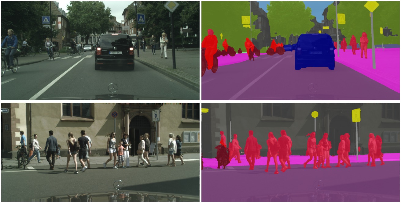
Convolutional networks, architectured to preserve spatial information in inputs through the use of local receptive fields, shared weights, and pooling layers, have been incredibly effective at learning representations from images and performing classification/regression tasks. While such networks are excellent at predicting a singular (or multiple) labels given an image, they are less suited for tasks such as semantic or instance segmentation, in which the expected output of an input image is a segmentation map highlighting different objects in the image (as in Figure 1).

Figure 1. An example of semantic segmentation, with input images at left and desired (segmented) outputs at right. Note that the semantic segmentation task does not require the output to differentiate between different members of the same class; all persons are highlighted the same color. Image due to (Kundu et al., 2016).

An obvious method to approach semantic segmentation with convolutional networks is with a sliding window; one can subsample a region of pixels around every given input pixel, pass that region as input to a convolutional network, and assign the prediction of the network to the input pixel’s location in the segmentation map. Doing so for every input pixel would indeed work, but would be incredibly computationally expensive, requiring one inference for each pixel.

Fully convolutional networks attempt to solve this problem by (a) replacing the fully connected layers in traditional convolutional networks with equivalent convolutional layers, and (b) introducing upsampling (transposed convolution) layers to ensure that the output is the same size as the original image. While (Long et al., 2015) introduce and describe both such modifications in their seminal work, the discussion is dense and leaves much to unpack—in this post, we’ll take a deeper dive into understanding the reasoning and implementation of fully convolutional networks.

Replacing Fully Connected Layers

While convolutional and pooling layers preserve spatial information with respect to the input, fully connected layers lose all such information by compressing previous layer activations into a single set of fully connected nodes. This loss of spatial information makes it impossible to create a one-to-one mapping between input and output pixels in a network with fully connected layers.

However, we can note that the only difference between fully connected and convolutional layers is that the neurons in a convolutional layer are only connected to a local region of the input (receptive fields) and that neurons associated with a feature map share parameters (parameter sharing).¹ Since the neurons in fully connected and convolutional layers still compute dot products, they share a functional form, and so it’s possible to convert between fully connected and convolutional layers.²

Precisely, we can convert fully connected layers to convolutional layers by replacing a fully connected layer with a convolutional layer that has a receptive field that spans all of the nodes in the previous convolutional layer. For example, if convolutional layer $l-1$ operating on a $224 \times 224$ input has output $[7 \times 7 \times 512]$ and is followed by 1000-dimensional fully connected layer $l$, an equivalent reformulation would be to replace $l$ with a convolutional layer with 1000 feature maps of size $d = 7$. Layer $l$ would therefore produce output of size $[1 \times 1 \times 1000]$, as desired.

But how exactly would replacing fully connected layers with convolutional layers benefit us? Say we replaced the input of layer $l-1$ with a $384 \times 384$ image; if a $224 \times 224$ image gives a volume of size $[7 \times 7 \times 512]$ (a reduction by 32), a $384 \times 384$ image will give a volume of size $[12 \times 12 \times 512]$ as $384/32 = 12$. While this would cause problems for a fully connected layer $l$, our modified convolutional layer $l$ will have an output of size $[6 \times 6 \times 1000]$ as $12 - 7 + 1 = 6$. As a result, instead of a single vector of class scores of length 1000, we obtain a $6 \times 6$ array of class scores across the $384 \times 384$ input image. This array corresponds to scores we would obtain were we to slide a $224 \times 224$ patch across the $384 \times 384$ image in striids of 32 pixels—but we obtain it in one forward pass!

Upsampling with Transposed Convolutions

So far, we’ve discussed the process of replacing fully connected layers with their convolutional layer equivalents, thus preserving spatial information. We can use this method directly to perform semantic segmentation: if all of the convolutions in our network are same convolutions as opposed to valid convolutions, our convolutional layers all operate on the full size of the image, allowing us to compute a pixel-wise mean squared error between the final output and the segmentation ground truth. However, the computational cost of developing a model only using same convolutions and never downsampling is incredibly high, making such an approach infeasible.

If we allow convolutional layers to downsample their input, we require the ability to upsample our outputs for final semantic segmentation. Traditional convolutional layers can’t do this for us, as they can only preserve input size or downsample. As a result, we’ll need a new tool to allow for upsampling.

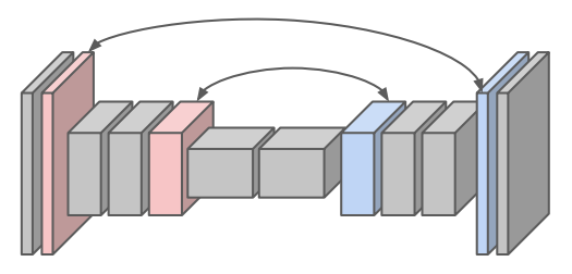
Fixed Upsampling. Consider a network that consisted only of same convolutions but downsampled with maximum pooling. An intuitive method to perform upsampling for this network is to introduce layers that perform the “opposite” of maximum pooling. Concretely, recall that maximum pooling selects the largest value in partitioned patches of its input and produces an output solely of those largest values, storing sentinels that record where the maximum values originated from (for the purposes of backpropagation). Maximum unpooling layers use the sentinels from their corresponding pooling layers to set the corresponding values at their locations before pooling, and set the remaining values to zero (see slide 19 for a visualization). Doing so is a reasonable attempt to “reverse” the pooling operations at later stages in the network, producing a model as in Figure 2.

Figure 2. An example of in-network upsampling. The colored layers represent pairs of maximum pooling/unpooling layers immediately followed by convolutions; the pooling/unpooling layers are responsible for changes in dimensionality, while all convolutions operate in same mode (and hence preserve dimensionality). The output shape is the same as the input shape, as desired.

Learnable Upsampling. In-network upsampling provides a promising approach for downsampling and upsampling within convolutional networks, but requires that all convolutions operate in same mode, with changes in dimensionality only occurring at pooling layers. It additionally defines a relatively simple function for upsampling, using no learnable parameters. Learnable upsampling provides a remedy for both of these approaches, defining a generalized layer that can perform upsampling in a backpropagation-amenable manner.

Recall that, in a general sense, the convolution operation defines a weight matrix $w$ which is multiplied with a patch of the same size from the input and summed to produce a weighted output. Learnable upsampling performs a very similar operation; it also defines a weight matrix $w$, but it instead performs elementwise multiplication of $w$ with each input value and combines the resulting outputs to produce a larger weighted output. This combination is performed by specifying a “stride” value, which indicates how much the output should be moved for each movement in the input; see Figure 3 for an example.

Figure 3. An example of learnable upsampling due to StackOverflow user andriys. Here, the image is the input to the upsampling layer and the filter is the weight matrix $w$, which is elementwise multiplied with each input value and combined according to a certain stride.

Let’s look more closely at the learnable upsampling operation.

• In the forward pass, this operation multiplies a single input value by a weight matrix and tiles the output values according to a stride. This is exactly what we do in the backward pass in a regular convolutional layer; we multiply a gradient value with its weighted connections to the previous layer to obtain the gradient of the previous layer.

• In the backward pass, this operation will backpropagate gradients by multiplying them with the weight matrix and summing contributions to arrive at the gradient for each input value. But this is exactly what we do in the forward pass of a regular convolutional layer; we elementwise multiply the weight matrix with a patch of the input and sum the resulting values.

These insights make it incredibly easy to implement learnable upsampling: we just switch the forward and backward passes of a normal convolution! So we can now make sense of the phrase used in Section 3.3. of (Long et al., 2015):

Upsampling is backwards strided convolution

Indeed, upsampling performs a “backwards” convolution according to a stride that defines how the output is tiled for movement in the input.

What’s in a name? The learnable upsampling operation has many names in literature, including deconvolution, upconvolution, fractionally strided convolution, and backward strided convolution. Deconvolution is a rather unfortunate name (as the upsampling layer doesn’t actually perform the deconvolution operation), but has stuck around for historical reasons. Upconvolution is used to refer to the fact that the output of a learnable upsampling layer is larger than the input. Fractionally strided convlution is used as strides often refer to how many input values are moved for every output value in a convolution operation, so learnable upsampling employs fractional strides (as multiple output values are moved for every input value).

Summary

Fully convolutional networks work due the (a) transformation of fully connected layers to spatially-aware convolutional layers and (b) introduction of (learnable) upsampling layers to allow for computational efficiency in producing an output of same dimensions as the input. As a result of these adjustments, such networks—true to their name—only use convolutional and pooling operations, discarding fully connected layers entirely.

Notes